15 Excel tips every SEO professional must know

Whether its basketball, pubic speaking, or SEO, mastering the fundamentals is key. Sure, you may be able to alter a data set manually or copy a strange looking formula, but if you want to be prepared for the challenges of tomorrow, this article will get you a long way.

Mikkel Sciegienny at Spreadsheeto has been involved with SEO for five years and in this blog post he will share 15 important tips for mastering Excel.

15 Excel tips every SEO professional must know

Excel is one of the most widely used software programs in the world, and is used in niches you can’t even think of. But in many niches and industries, there are work processes that scream for Excel.

One of the common factors for these work processes is that they include a lot of data that sometimes needs to be cleaned up before it makes sense. Other common factors are keeping track of stuff like emails, replies and links. Lots of links.
Luckily there’s a tool that’s so powerful and flexible that it covers all this – can you guess what software program I am talking about?
As an SEO professional, Excel skills can ease up your work and increase your productivity – which will make you an even better SEO.

In this article, I’ll teach you the tips you need to know to improve your Excel skills in a matter of minutes. This article and the examples are written for Excel 2016 on a machine running Windows, but almost all of the tips are universal for Excel 2007/10/13/16 for Windows, although the layout may look a bit different on your version.
We start off with the easy tips and progress to the more advanced ones.

Tip 1 - Freeze panes:

Don’t lose track of your headers

When working with tons of rows and columns, freezing the column headers will make it a lot easier to keep track of the data you’re looking for.
Scroll to the top of your spreadsheet. Go to the ‘View’ tab on the ribbon (that’s the fancy word for the menu with all the buttons by the way). Then click the ‘Freeze Panes’ button.
Now click the ‘Freeze Top Row’ option.

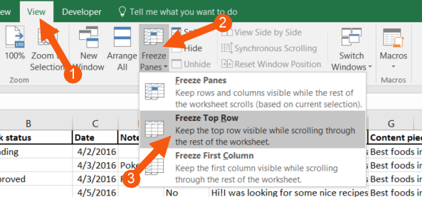
When you’ve done this, try to scroll down your sheet. You now see that the headers in row 1 follow along as you scroll down the spreadsheet.
This means that from now on, you never have to scroll to the top of your sheet to see what columns you’ve selected when you’re in in a row below the fold. And when working with SEO, you will encounter this issue sooner or later.

Tip 2 - Wrap Text:

Inserting long texts nicely

The content of a cell can be too big to fit in it properly. This is particularly true when dealing with longer strings of texts, e.g. email text for outreaching.
When copied directly into Excel the cell is by default automatically fitted to the text. That means it can ruin the design of your spreadsheet because it gets absurdly large.
When this happens, left-click the name of the column (A, B, C, D…) right above row 1 that holds the cells with a lot of text.
Then click the ‘Wrap Text’ button on the ‘Home’ tab of the ribbon so it’s deselected.

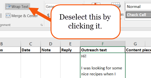
Now your text looks like it’s “hidden” behind the other cells. This is a good thing since it now doesn’t break the layout of the sheet by oversizing the rows.

Tip 3 – Paste as values:

When you just need the formula results

Copying and pasting are some of the most used features of a computer – and of course also in Excel. Pasting values only, when copying cells that include formulas, makes it possible for you to easily relocate values in your spreadsheet.
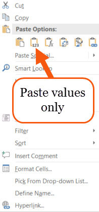
After you’ve copied one or more cells then, when pasting the cells, right click the desired destination of cells and look to the ‘Paste Options:’.
The second option here is called ‘Values (V)’ (which you’ll see when you hover your mouse over it). Click it, and the copied cells are now inserted as values instead of whatever they were before.

This is especially useful when you’ve done some calculations on rankings, CTR or conversion rates and need to relocate the results of your formulas.

Tip 4 – Filters:

Cut out the data you don’t need

Filters are one of the most loved features of Excel, both for its ease of use and its ability to get what you want from your massive datasheet in no time. As an SEO expert filtering in Excel is a must-know.
First, select any cell within your data.
Then click the ‘Data’ tab on the ribbon and click the ‘Filter’ button.
Now you’ll see a drop-down button next to each of your column headers.

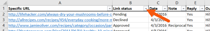
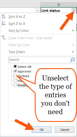
When you click these buttons, you have options to filter out which rows you want and don’t want to see. When unselecting one, or more, of the options and clicking ‘OK’, the rows that contain that specific data in that specific column will not be shown.
This is also applicable the other way around. E.g., if you only want to see the rows with links that have been approved, then uncheck all the other checkboxes and click ‘OK’. Then you’ll only see the rows where the ‘Link status’ is “Approved.” The other rows will be hidden.

Tip 5 – Remove Hyperlinks:

Convert multiple hyperlinks to regular text in seconds

As a default, Excel recognizes text that starts with http:// as a hyperlink. That means that Excel automatically gets the blue font color and the underlining and when you click it, it opens in your default browser.
When keeping track of data with a lot of links all these hyperlinks are not very beneficial to you. It’s much easier if they were just regular text.
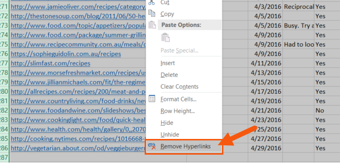
You can convert all your hyperlinks to text at once by pressing the shortcut ‘Ctrl + A’ twice to select all the cells in your sheet.
Then right-click any cell and click ‘Remove hyperlinks’.

Tip 6 – Find and Replace:

The quickest way to clean up data

The ‘Find and Replace’ feature is one of Excel’s most underused features. Most Excel users don’t imagine using it to clean up parts of a lot of text strings at once.
A great example of this is a situation where you want to remove the “www.” part of all your URLs.
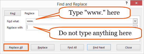
Select the column that holds your URLs by left-clicking the column name right above row 1. Then use the shortcut ‘Ctrl + H’ to bring up the ‘Find and Replace’ dialog box.
In the ‘Find what:’ field type in “www.” and do nothing else. Then click ‘Replace All’.

Now you’ve removed all instances of “www.” From all URLs in that column. Rinse and repeat as needed.
This is by far the fastest way of cleaning up URLs in Excel.

Tip 7 - Import a .CSV file:

Using your Excel skills on your exports.

Many SEO-tools like AHREFS, Google Analytics, SEMrush, etc., makes it possible for you to export your findings to a .CSV file. When you open that file in Excel, you can do all the manipulation with it you want. However, opening a .CSV-file is not as straightforward as it sounds. There’s a few things you need to be aware of.
Open a blank Excel sheet, then click the ‘Data’ tab on the ribbon and click the button that says ‘From Text’.

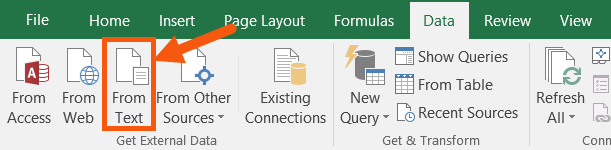
Find your .CSV-file in the browser window and hit ‘Open’.
Now a series of dialog boxes called ‘Text Import Wizard’ appears. This wizard will take you through 3 steps where 2 of them are unnecessary.
If you’ve exported as a .CSV from the above-mentioned programs, then your .CSV- file is very standard and you can just click the ‘Next >’ button in step 1 of 3.
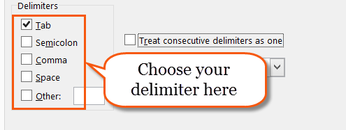
In step 2 of 3, you simply choose the delimiter. It’s not always comma separated. Sometimes the data is separated by a semi-colon or just a tab. If you’re unsure about which delimiter to use, then look at the ‘Example’ window and try to click through them all to see which one that fits the data.

You can skip the entire step 3 of the ‘Text Import Wizard’ and just go ahead and click the ‘Finish’-button.
You may or may not get a new dialog box that asks you where you want to put this freshly imported data. I usually just click ‘OK’ as it’s defaulted to choose cell A1.
And there you have it, as CSV-file imported, correctly, in the matter of seconds.

Tip 8 – Conditional formatting:

Identifying duplicates

Conditional formatting is used for coloring your sheet if certain conditions are met. When you type in a new entry in your outreach sheet, you instantly need to know if you’ve already sent an email regarding this specific URL before.
Select the entire column with your URLs by clicking on the name of the column (A, B, C, D…) just above row 1.
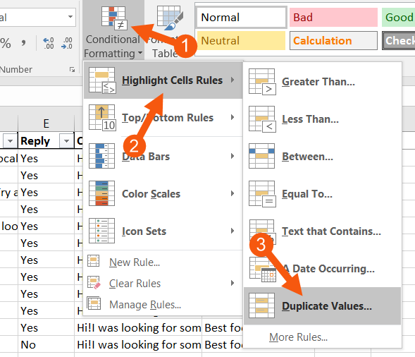
Then click the ‘Conditional Formatting’ button on the ‘Home’ tab of the ribbon. Hover your mouse over ‘Highlight Cells Rules’ and chose ‘Duplicate Values…’

Click ‘OK’ to the next dialog box (or chose custom formatting by clicking the dropdown and selecting ‘Custom Format…’) and then watch out for those colored duplicate values in your column.

Tip 9 – Remove Duplicates:

Continuing where we left off.

If you don’t need to look through your duplicates by eye, then Excel can do the job of removing them for you.
Select any cell in your data, then go to the ‘Data’ tab of the ribbon and click ‘Remove Duplicates’.
In the dialog box that appears, you can choose how strict you want Excel to be when removing the duplicates. If you leave all the checkboxes checked then Excel will only remove the entries that match another entry in all cells in the row (within the columns of the data).

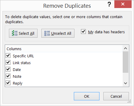
If you click ‘Unselect all’ and in this example check the ‘Specific URL’ checkbox, then Excel will only remove entries where the column with URLs match another entry’s URL.
Note: If Excel finds a duplicate it will remove the entire row, no matter how many checkboxes you’ve checked.

Tip 10 – Data validation:

Use a dropdown to control what’s in the cells

Analysis of your work gets a lot easier if you control the variety of cell input. Summing up on ‘Link status’ is time-consuming if you’ve built an outreach sheet of more than a thousand entries and haven’t had a systematic approach to what you enter in the cells.
To avoid dealing with permutations of words like “Approved”, “Declined” and “Pending”, use a drop-down menu to control the input.
Create a new sheet by using the shortcut ‘Shift + F11’. In the new sheet write all the things that you want to be able to choose from in the drop-down menu.
Go back to your original sheet and select all the cells you want to have in the drop-down menu. Then go to the ‘Data’ tab in the ribbon and click the ‘Data Validation’ button.

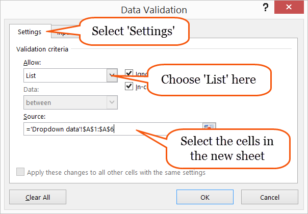
In the dialog box be sure to be in the ‘Settings’ tab. Then under ‘Allow:’ choose ‘List’ and then choose the source for your drop-down menu. The source data is the cells that holds the drop-down menu options in the new sheet you just created earlier.
Click ‘OK’ and then you’re good to go with a drop-down menu that keeps your data simple and ready for analysis.

Tip 11 – VLOOKUP:

Find a cell somewhere else and bring back corresponding data

You might’ve heard about the famous ‘VLOOKUP-function’ before. As far as usability goes, ‘VLOOKUP’ has definitely earned the hype.
Imagine having two sheets of data. One to keep track of outreach and one where you’ve imported a massive export from your keyword miner that, among much else, holds the Domain Authority (DA) for 10,000 interesting URLs.
Now you want to get that DA from that sheet to your outreach sheet on all entries.
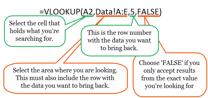
‘VLOOKUP’ basically consists of four things:

1) The value you’re looking for.
2) The area where you are looking.
3) The data you want to bring from the area you are looking.
4) A choice of how precise in your search you want to be.

These four things are a simple explanation of what is normally called the ‘syntax’ of an Excel function. And this is how you use the function:

This is the quick way of learning and using ‘VLOOKUP’. There’s so much more to VLOOKUP, and I highly suggest you get yourself familiar with this function.

Tip 12 – COUNTIF:

Count cells if they meet certain criteria

Summarizing data is necessary for you to evaluate your work. In SEO, that usually comes to show in form of counting stuff. E.g. counting how many of your outreach emails that resulted in a link.
The ‘COUNIF-function’ is very simple to use. It consists of:

1) Where you want to count.
2) What you want to count.

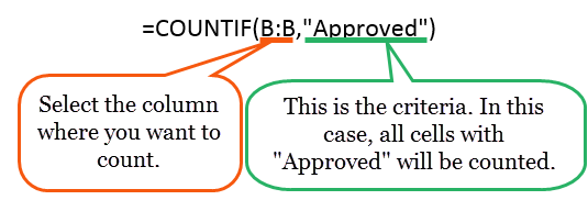
You can exchange the column where you want to count and the criteria to match your data. Remember to put text criteria in double quotes. If you’re counting specific values and not text, just type in the number.
‘COUNTIF’ is a deeper subject than what I’ve just showed you here. Check out this video by ExcelIsFun that explains 21 different examples of ‘COUNTIF’-usage.

Tip 13 – IFERROR:

Cleanup formulas that don’t give you answers

When a formula can’t give you a result it spits out an error (usually looks like #N/A). There can be multiple causes for a formula to return an error but usually, it’s because a ‘VLOOKUP’ can’t find the value you’re looking for or a ‘COUNTIF’ can’t find any cells with the criteria you’ve given.
Sometimes you will look at these errors and fix them – but sometimes they require no fix. If you keep the formulas with errors, you have to look at those ugly cells with #N/A. And they don’t look pretty.
You can remove the errors from sight by using the ‘IFERROR-function’. It’s very easy to use and consists of 2 things:

1) The formula you are using.
2) What you want instead of a potential error.
Here’s how you use ‘IFERROR’:

Remember that the ‘IFERROR-function’ can be used before any other function or combination of functions. You can even put another function instead of the above “Can’t find” if you need a calculation or lookup to be made if the first function doesn’t give a result.

Tip 14 – Charts:

Visualizing your SEO work

Visual overviews are always easier to read and tells you what you want to know faster than just numbers. You can feed the results from your ‘COUNTIF-functions’ into a chart to get a nice looking overview of what’s going on in your spreadsheet.
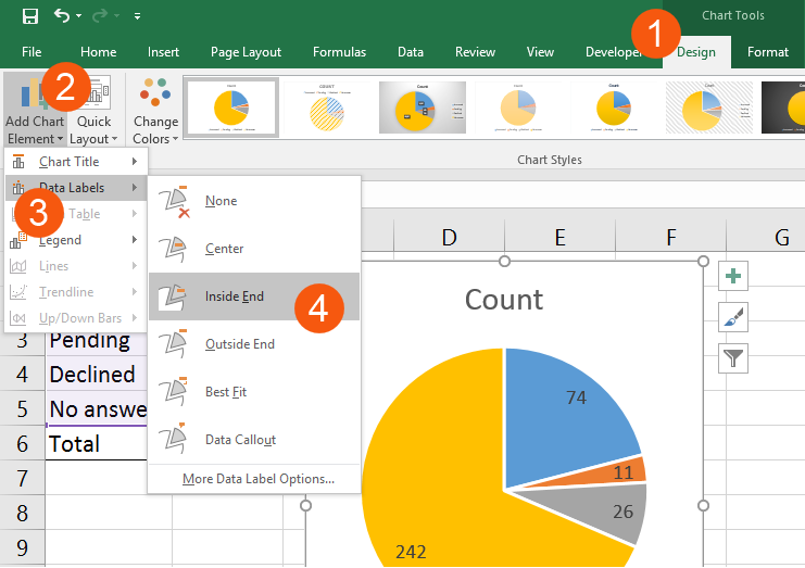
If you’ve counted your outreach progress using the ‘COUNTIF-function’ let’s throw that data into a pie chart.
Select your headers, categories and counts like the example below. Then click the ‘Insert’ tab of the ribbon and click the button that looks like a pie chart. Choose your desired design.

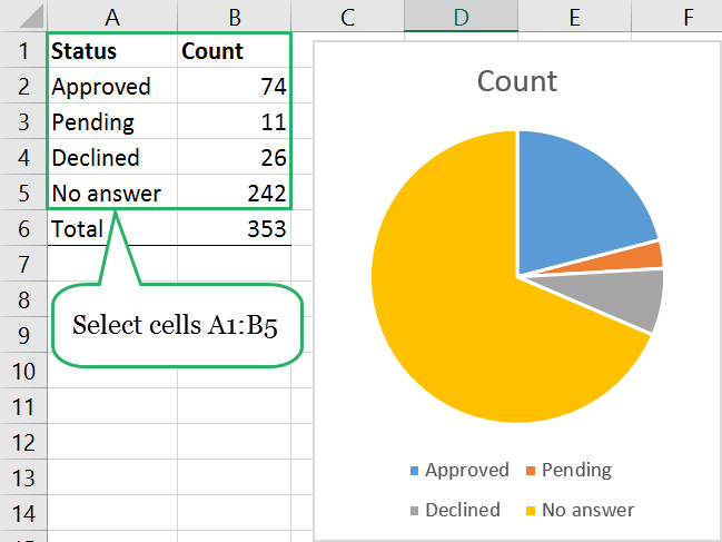
You can modify the chart to your needs by using the two new tabs that appear when you select the chart. From the ‘Design’ tab, you can easily add some data labels if you think the chart’s not precise enough.

Tip 15 – VBA:

Macro to make URLs active.

When you have lots of inactive URLs in your spreadsheet (maybe they’re inactive because you removed the hyperlinks with help from Tip 5) there’s only one way to make them all active at once: VBA.
The programming language Visual Basic for Applications offers a solution to any Excel challenge, but it requires some skill to use. In this case, you don’t have to worry - I’ve done all the work for you.

1) Use the shortcut Alt + F11 to open up the VBA-editor.
2) Click ‘Insert’ and then click ‘Module’.
3) Copy the code from below and insert it here.
4) Close the VBA-editor (click the cross in the upper right corner of the window).

Here’s the code:

Sub Activatelinks()
    Dim cell As Range
    For Each cell In Selection
        cell.Hyperlinks.Add Anchor:=cell, Address:=cell.Text
    Next cell
End Sub

Now select the cells with the URLs you want to activate and go to the ‘View’ tab of the ribbon. From here you click the ‘Macros’ button.
Select the ‘Activatelinks’ macro and hit ‘Run’.
Try to click the hyperlinks that are now underlined and colored blue as a hyperlink usually is.

Check out more content of Mikkel Sciegienny at Spreadsheeto or contact him at
mikkel@spreadsheeto.com